2.2. Decay Chain Worked Examples

This page works a decay-chain problem in each direction: first forward — modeling the production and decay of ²²⁵Ra, a generator of the medical isotope ²²⁵Ac — and then inverse — fitting the activity of the ¹⁵²Eu source measured in the Spectroscopy Worked Examples, and checking it against the source’s certificate.

Forward: producing 225Ra

Suppose a target is irradiated for 4.5 days, producing ²²⁵Ra (half-life 14.9 d), but the beam current varied: the production rate was 9 atoms/s for the first half day, dropped to 2/s for the next day, and recovered to 5/s for the remaining three days. This piecewise-constant history is exactly what the R argument describes — each row is [rate, time] with time the end of that interval:

import curie as ci
import numpy as np

dc = ci.DecayChain('225RA', R=[[9, 0.5], [2, 1.5], [5, 4.5]], units='d')
print(dc.isotopes)

['225RAg', '225ACg', '221FRg', '217ATg', '213BIg', '217RNg',
 '209TLg', '213POg', '209PBg', '209BIg', '205TLg']

Curie followed the decay data all the way to stability: the chain includes ²²⁵Ac and its short-lived descendants down to stable thallium and bismuth. Plotting shows the whole history — production before t = 0, decay after:

dc.plot(time=np.linspace(0, 40, 500), max_plot=5)

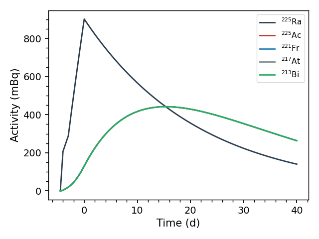
The parent’s activity peaks at the end of bombardment (t = 0), while ²²⁵Ac grows in for about two weeks afterwards — the daughters sit on a common curve because the sub-²²⁵Ac chain reaches equilibrium within hours. Any single value is available directly, in the chain’s units (days here):

>>> print(dc.activity('225AC', time=10))
0.4168212066113324
>>> print(dc.R_avg)
  isotope     R_avg
0  225RAg  4.777778

If measured counts of any chain member are available, dc.fit_R() rescales this production history to match them (the shape — the beam’s ups and downs — is preserved; only the overall scale is fit).

Inverse: how active was the 152Eu source?

The Spectroscopy Worked Examples calibrated a detector with a ¹⁵²Eu source certified at 37.0 kBq on 01/01/2009, using a spectrum counted in 2018. Here we ask the reverse question: given only that spectrum’s fitted peaks, what was the source activity on the certificate date?

Starting from the calibrated spectrum sp of the Spectroscopy Worked Examples, build a decay-only chain (an A0 guess rather than a production history) and load the measured decays from the spectrum. The certificate date is our t = 0, passed as the EoB (end-of-bombardment) argument — despite the name, it is simply the t = 0 reference time, even when, as here, nothing was bombarded:

dc = ci.DecayChain('152EU', A0=3.7E4, units='y')
dc.get_counts([sp], EoB='01/01/2009 12:00:00')

get_counts() took each fitted gamma line’s decays from sp.peaks and placed the count interval on the chain’s clock — 9.7 years after t = 0:

>>> print(dc.counts[['isotope', 'start', 'stop', 'counts', 'unc_counts']].head(3))
  isotope     start      stop        counts    unc_counts
0  152EUg  9.697086  9.697163  5.537235e+07  1.366835e+07
1  152EUg  9.697086  9.697163  5.576780e+07  8.454064e+06
2  152EUg  9.697086  9.697163  4.874544e+07  1.161682e+07

(The same works without the live spectrum: get_counts also accepts the peak file saved in the Spectroscopy Worked Examples, as dc.get_counts(['eu_calib_7cm.Spe'], EoB=..., peak_data='eu_peaks.csv').) Now fit the initial activity:

>>> isotopes, A0_fit, cov = dc.fit_A0()
>>> print('{:.3g} +/- {:.2g} Bq'.format(A0_fit[0], np.sqrt(cov[0][0])))
3.63e+04 +/- 2.5e+03 Bq

and plot the fitted decay curve against the measurements:

dc.plot(max_plot=1, max_plot_error=0.2)

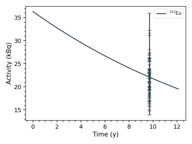
The fitted activity at the certificate date is 36.3 +/- 2.5 kBq — in agreement with the certified 37.0 kBq. Each point in the plot is one gamma line’s estimate of the activity; the fit combines them while accounting for their shared uncertainties, the efficiency calibration and the line intensities. Shared errors cannot be averaged away by adding more lines, so the combined uncertainty is larger — and more honest — than a naive average of the points would suggest.

Here the source decayed freely, so fit_A0() was the right tool. In an activation experiment you would instead give the chain your estimated production history R and call fit_R() — everything else, get_counts() included, works the same way.