3. Reactions
Curie provides evaluated nuclear reaction cross sections through two
classes: the Reaction class holds the cross section for one specific
reaction — its energy grid, values, uncertainties (where available), and
methods to interpolate, flux-average and plot — and the Library class
searches the underlying data libraries for what reactions exist.
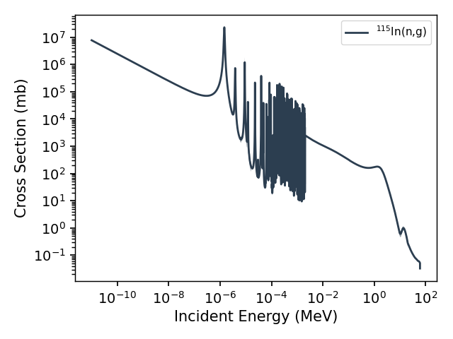
The 115In(n,g) capture cross section (IRDFF-II), across ten orders of magnitude in incident energy.
Reactions are named in standard nuclear reaction notation — the pattern
is TARGET(incident,outgoing)PRODUCT, with isotopes written in either
of Curie’s name forms:
rx = ci.Reaction('115IN(n,g)')             # neutron capture on 115In
rx = ci.Reaction('Ra-226(n,2n)Ra-225')     # (n,2n), naming the product
rx = ci.Reaction('natTI(p,x)48V')          # any route from natural Ti to 48V
All cross sections are in mb, and all energies in MeV.
Workflow. Using reaction data usually takes three steps:
Find the reaction. If you know its name, construct it directly; if not,
Library.search()lists what a library contains (ci.Library('iaea').search(target='natTI', incident='p')).Choose the source. By default (
library='best') Curie picks the highest-priority library carrying the reaction; pass a library name to choose yourself.rx.library.namealways reports which library was selected.Use the data:
rx.interpolate(energy)for values on your own energy grid,rx.average(energy, flux)for the flux-averaged cross section of a measurement,rx.plot()to look at it.
See the Reaction How-to Guide for each step in detail, the Reactions Worked Examples for a complete monitor-reaction example with library comparisons, and Reactions Troubleshooting for the common failure modes.
Uses and limitations. These are evaluated libraries — smooth, recommended curves produced by evaluators from experimental data and nuclear-model calculations — not raw experimental data points (EXFOR, the international compilation of such measurements, is not included). Each library has a scope and a character: the IAEA library is a set of precisely evaluated monitor (beam-normalization) reactions with uncertainties; IRDFF-II is a neutron-dosimetry standard, also with uncertainties; ENDF/B-VIII.1 is the general-purpose neutron evaluation; and the TENDL-2025 libraries are theory-driven (TALYS-based) evaluations whose strength is complete coverage — nearly every target and product, including reactions no one has measured. Where they overlap, they will not agree perfectly; which to prefer, and what to watch out for (energy-grid limits, natural vs isotopic targets, cumulative vs direct/independent production), is covered in the Reactions Worked Examples.
Averages vs. integrals. Reaction offers two ways to combine a cross section with a particle
spectrum, and which one you want depends on what your flux array means:
rx.average(eng, phi)returns the flux-weighted average cross section \(\langle\sigma\rangle\), in mb. Only the shape ofphimatters — its normalization cancels — so this is the right tool when the spectrum is relative: the energy distribution of beam particles in a foil fromStack, for example, or any spectrum you know only up to a constant. The absolute physics then enters through numbers you know separately. For a thin target in a charged-particle beam, the production rate thatDecayChaintakes as itsRinput is\[R \;[\mathrm{atoms/s}] = I_p\,n_t\, \langle\sigma\rangle \times 10^{-27}\]with \(I_p\) the beam current (particles/s), \(n_t\) the areal number density of target atoms (atoms/cm2), and \(10^{-27}\) converting mb to cm2. (Note \(n_t\) is atoms per area — from a foil’s areal density in mg/cm2, as
Stackreports it, multiply by \(10^{-3} N_A / M\) with \(M\) the molar mass in g/mol.)rx.integrate(eng, phi)returns the flux integral \(\int \sigma(E)\,\phi(E)\,dE\). Here the normalization ofphiis the point: give an absolute differential flux (particles per cm2 per second per MeV) and the integral is proportional to the reaction rate per target atom (raw units mb/cm2/s) — multiply by \(10^{-27}\) to convert mb to cm2, giving the per-atom rate in 1/s, and by the number of target atoms for the production rate. This is the natural form for yield calculations in a fully specified field, such as a reactor neutron spectrum quoted as a differential flux.
The two are related by the total flux —
integrate(eng, phi) = average(eng, phi) * sum(phi*dE) — so this is
one calculation viewed two ways: use average when the shape and the
magnitude of your flux come from different places, and integrate
when one spectrum carries both.