Quickstart

Once Curie is installed (see Installation), everything is reached through a single import:

import curie as ci

This page maps out the toolkit — which class does what, and where to read more — and gives a few short examples to run.

The Curie toolbox

Curie’s functionality lives in a handful of classes, grouped here by what you would use them for. The classes are designed to work together: peaks fit from a spectrum feed a decay-chain fit, a foil’s particle flux feeds a cross-section average, and so on.

Fitting gamma-ray spectra. Spectrum fits the peaks in HPGe (high-purity germanium) detector data, using a Calibration (energy, efficiency and resolution) and Isotope decay data to turn peak areas into activities. See Spectroscopy.

Production and decay calculations. Isotope provides decay data — half-lives, decay radiations, dose rates — for a single nuclide, while DecayChain solves the Bateman equations for a whole chain: forward (predicting activities from a production rate) or inverse (fitting a production rate or initial activity to measured decays, including peaks read straight from a Spectrum). See Isotopes & Decay Chains.

Nuclear reaction data. Reaction gives a cross section as a function of energy, with interpolation, flux-averaging and plotting; Library searches the evaluated libraries (ENDF, TENDL, IRDFF, IAEA) for what is available. See Reactions.

Stopping powers and stacked targets. Element and Compound compute charged-particle stopping powers, ranges and photon attenuation coefficients; Stack transports a beam through a stack of foils to find the particle energy in each — a flux that can be handed straight to Reaction.average. See Stopping Power Calculations.

For the models and formulas behind these methods, see the Theory & Methodology chapter; for every method and attribute, the API.

A few things to try

The first two examples need no local files — Curie fetches the nuclear data they use on first access.

Look up the decay data for a radionuclide:

>>> ip = ci.Isotope('225RA')
>>> print(ip.half_life('d'))
14.9
>>> print(ip.gammas())          # energies (keV) and intensities (%)
   energy  intensity  unc_intensity
0    40.0       30.0            1.5

Plot an evaluated reaction cross section (this one resolves to IRDFF-II):

rx = ci.Reaction('115IN(n,g)')  # neutron capture on 115In
rx.plot(scale='loglog')

The third fits peaks in a real gamma-ray spectrum, so it needs a data file. Download eu_calib_7cm.Spe from the examples directory of the repository and run from the folder you saved it in (or point the path at your own .Spe, .Chn, .CNF or .IEC spectrum):

sp = ci.Spectrum('eu_calib_7cm.Spe')
sp.isotopes = ['152EU']
sp.plot()                       # the spectrum, with its fitted peaks

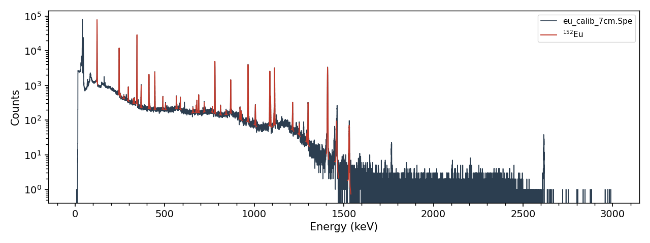
The fitted ¹⁵²Eu spectrum the code above produces.

Each links to a fuller, worked walk-through: Spectroscopy, Isotopes & Decay Chains, Reactions.

Example scripts

Complete, runnable scripts covering each of these areas ship in the examples directory of the Curie repository, alongside the example data files they use.