3.2. Reactions Worked Examples

This page works through the reaction data behind a typical charged-particle activation measurement — a monitor reaction — and uses it to show how the libraries differ, and why those differences matter: natural versus isotopic targets, cumulative versus direct production, and the limits of each library’s energy grid.

A monitor reaction

In a stacked-target irradiation, thin foils of well-studied materials are interleaved with the samples: the activities induced in these monitor foils, together with precisely evaluated cross sections, measure the beam current and energy in each position. The IAEA maintains the reference library for exactly this purpose, and it is where Curie’s default library search sends charged-particle reactions:

>>> import curie as ci
>>> import numpy as np

>>> rx = ci.Reaction('natTI(p,x)48V')
>>> print(rx.library.name)
IAEA CP-Reference (2017)

Note the notation: a natural titanium target (natTI — monitor foils are natural metal), and (p,x) — any reaction route that ends at ⁴⁸V. The IAEA library provides uncertainties, so the flux-averaged cross section of a measurement comes with an error bar. For a proton spectrum centered at 20 MeV:

>>> eng = np.linspace(10, 30, 50)
>>> phi = np.exp(-0.5*((eng - 20)/3.5)**2)
>>> print(rx.average(eng, phi, unc=True))
(115.2..., 5.2...)

Natural vs. isotopic targets

The TENDL-2025 residual-product libraries carry this reaction for the natural target directly — natTI(p,x)48V works there just as it does in the IAEA library. The natural-element entries are abundance-weighted sums of the isotopic tables, computed when the databases are built:

r_nat = ci.Reaction('natTi(p,x)48Vg', 'tendl_p')

(The explicit g on the product picks the ground state — leaving it off works, but prints the ground-state-assumed warning.)

The weighted sum is also easy to carry out by hand, which shows exactly what the natural entry is. ci.Element('Ti').abundances provides the table the sum needs — the stable isotopes with their percent abundances (columns isotope and abundance):

el = ci.Element('Ti')
eng = np.linspace(1, 100, 500)
xs_nat = np.zeros_like(eng)

for n, row in el.abundances.iterrows():
        try:
                r = ci.Reaction('{0}(p,x)48Vg'.format(row['isotope']), 'tendl_p')
        except ValueError:
                continue      # this isotope has no route to 48V
        xs_nat += 1E-2*row['abundance']*r.interpolate(eng)

The try/except is doing real physics: ⁴⁶Ti + p has only 47 nucleons, so it cannot make ⁴⁸V at any energy, and TENDL has no such entry. Overlaying the natural-target entry on the IAEA evaluation:

f, ax = rx.plot(return_plot=True, label='library')
ax.plot(eng, r_nat.interpolate(eng), ls='--', label='TENDL-2025 (natural target)')
ax.legend()

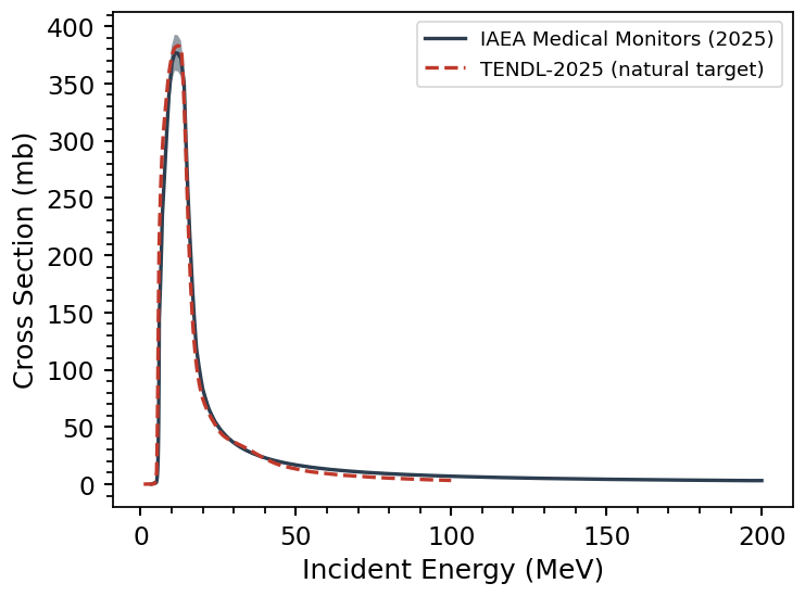
The two agree in shape, and for this reaction within ~1% at the peak — closer than is typical. The distinction still matters, and it reflects what each library is: the IAEA curve is an evaluation of decades of monitor-foil measurements; the TENDL curve comes from nuclear-model (TALYS) calculations, whose strength is covering every reaction — including ones never measured — rather than pinpoint accuracy on any one. For beam monitoring, use the IAEA values.

Cumulative vs. direct production

A subtlety of residual-product data: does “production of X” include the decay of short-lived parents into X, or only X made directly? The IAEA library distinguishes the two where it matters. For ¹⁷⁷Lu — the therapy isotope — produced by deuterons on ¹⁷⁶Yb, both are evaluated:

ra = ci.Reaction('176YB(d,x)177LUg', 'iaea')   # cumulative
rb = ci.Reaction('176YB(d,n)177LUg', 'iaea')   # direct only

f, ax = ra.plot(return_plot=True, label='reaction')
rb.plot(f=f, ax=ax, label='reaction')

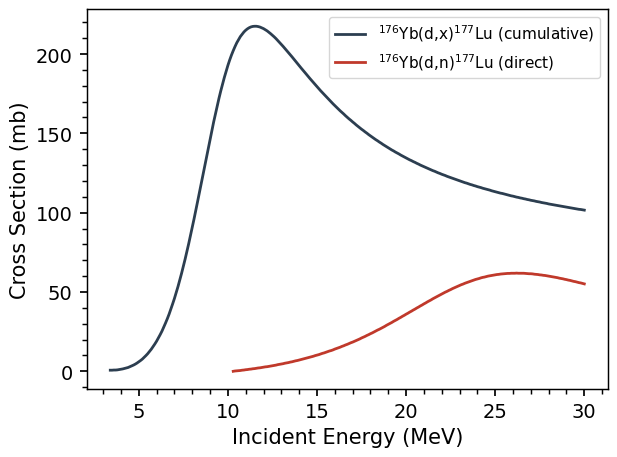
The cumulative curve — here several times the direct one — includes ¹⁷⁷Yb, which is also made by the beam and decays entirely to ¹⁷⁷Lu with a 1.9 h half-life. After a few hours of cooling, the cumulative cross section is what an activity measurement of ¹⁷⁷Lu actually sees. TENDL’s residual-product entries are, by contrast, independent: each state’s direct production only, with decay feeding left to you (DecayChain does exactly that bookkeeping — see Isotopes & Decay Chains). When comparing libraries or using a cross section to predict an activity, always ask which convention you are holding.

Neutron libraries and the 20 MeV cutoff

The same look-before-you-use advice applies to energy grids. Most ENDF/B-VIII.1 neutron evaluations stop at 20 MeV; IRDFF-II extends its dosimetry reactions to 60 MeV:

r1 = ci.Reaction('90ZR(n,2n)', 'irdff')
f, ax = r1.plot(return_plot=True, label='library')
r2 = ci.Reaction('90ZR(n,2n)', 'endf')
r2.plot(f=f, ax=ax, label='library')

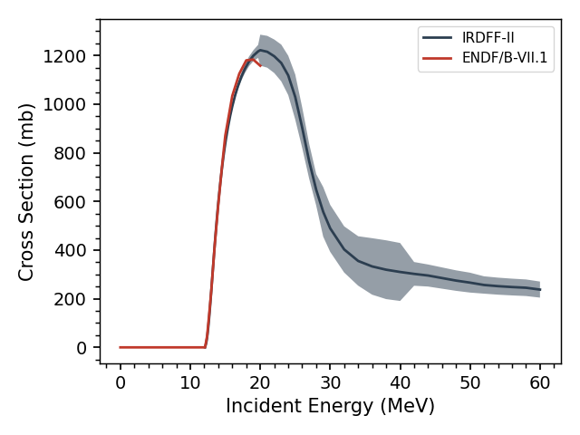
The two agree where they overlap — but the ENDF curve simply ends at 20 MeV, in the middle of the peak. Beyond a library’s grid Curie returns zero rather than extrapolating, so a flux average silently loses whatever part of the spectrum the library doesn’t cover. For a flat 12–30 MeV flux:

>>> eng = np.linspace(12, 30, 50)
>>> print(r1.average(eng, np.ones(50)))   # IRDFF-II
885.1...
>>> print(r2.average(eng, np.ones(50)))   # ENDF: zero above 20 MeV
362.6...

Same reaction, same flux — and a factor of 2.4 between the answers, entirely from the grid. Whenever your spectrum extends above ~20 MeV, check the reaction’s .eng.max() against it, and prefer IRDFF-II (or TENDL, which extends to 200 MeV) for the high-energy part.