1.2. Spectroscopy Worked Examples
This page walks through a complete efficiency calibration using
eu_calib_7cm.Spe — a spectrum of a 152Eu reference source
counted 7 cm from an HPGe detector, available in the examples folder of
the Curie repository. The source had a certified activity of 37.0 kBq
(1.0 uCi) on 01/01/2009.
Loading and inspecting the spectrum
Load the spectrum and plot the raw histogram:
import curie as ci

sp = ci.Spectrum('eu_calib_7cm.Spe')
sp.plot(fit=False)
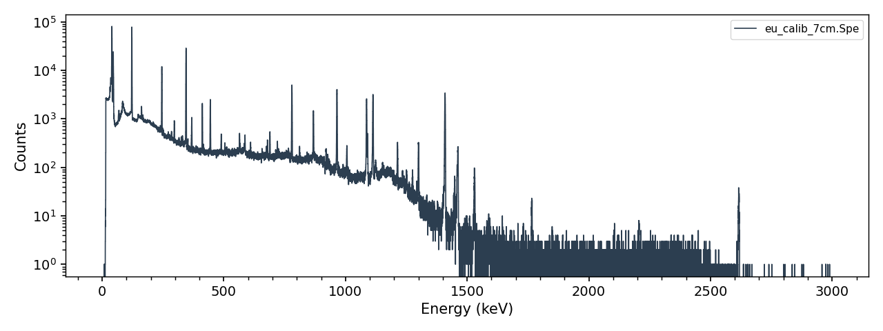
The energy calibration stored in the .Spe file header was read automatically:
>>> print(sp.cb.engcal)
[3.3973e-01 1.8297e-01 5.5683e-09]
Fitting the peaks
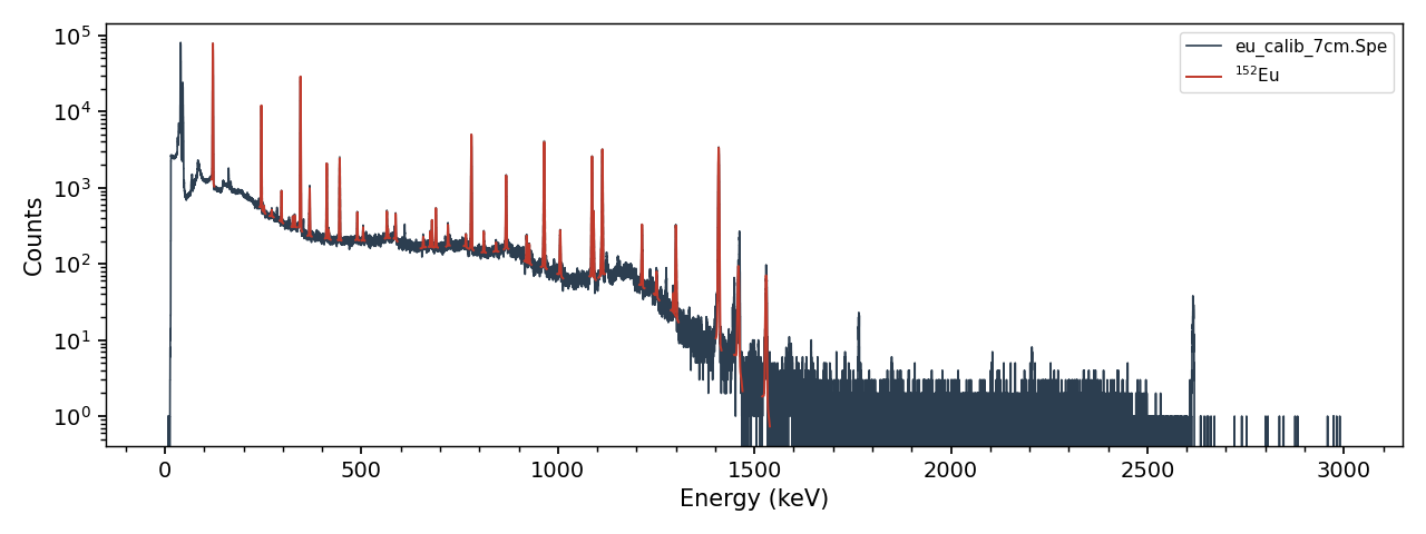
Tell Curie which isotopes are present, and it will fit every 152Eu line that passes the selection criteria (see Spectroscopy How-to Guide):
sp.isotopes = ['152EU']
sp.plot()
Fitting the efficiency calibration
The peak counts are correct at this point, but the decay rates are not: they are computed with the built-in default efficiency curve, not one measured for this detector. Calibrating requires the reference activity and date of the source:
cb = ci.Calibration()
cb.calibrate([sp], sources=[{'isotope':'152EU', 'A0':3.7E4,
                             'ref_date':'01/01/2009 12:00:00'}])
cb.plot()
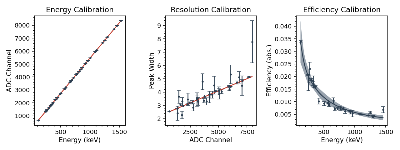
calibrate() refit the energy, resolution and efficiency calibrations
from the fitted peaks (the procedure and functional forms are described in
Detector Calibration), and applied them to the spectrum. The fitted
efficiency parameters (and their uncertainties) are stored on the
calibration:
>>> print(cb.effcal)
[5.02300989e-02 1.00000000e+02 2.82394962e+00 2.45721823e+00
 2.91455256e-01]
Checking the results
With the calibration applied, the peak table now reports consistent decay rates across lines spanning 122 to 1408 keV:
>>> print(sp.peaks[['isotope','energy','counts','unc_counts','intensity',
...                 'efficiency','decay_rate','unc_decay_rate','chi2']].head(8))
  isotope    energy    counts  unc_counts  intensity  efficiency  decay_rate  unc_decay_rate   chi2
0   152EU  121.7817  498786.0      3118.0   0.285300     0.03385     22564.0          5570.0  20.18
1   152EU  244.6974   80193.0       403.0   0.075500     0.02042     22725.0          3445.0   1.96
2   152EU  251.6330     610.0       112.0   0.000670     0.02002     19864.0          4734.0   1.96
3   152EU  271.0800     853.0        93.0   0.000715     0.01903     27381.0          4856.0   0.93
4   152EU  295.9387    4258.0        98.0   0.004400     0.01792     23594.0          2803.0   0.90
5   152EU  324.8300     642.0        64.0   0.000681     0.01676     24556.0          3486.0   0.92
6   152EU  329.4100    1055.0        78.0   0.001213     0.01659     22900.0          2792.0   0.92
7   152EU  344.2785  213990.0       669.0   0.265900     0.01605     21911.0          2030.0   2.19
The decay_rate column — the activity of the source during the count —
clusters around 22.6 kBq for every line: the 37.0 kBq source decayed for
9.7 years — a bit under one 13.5 y half-life — between the reference
date and the count.
(The large chi2 on the very intense 122 keV peak is expected for a
peak with half a million counts — see the note on high-statistics peaks in
Spectroscopy Troubleshooting.) sp.summarize() prints the same
information line by line:
>>> sp.summarize()
...
152EU - 244.6974 keV (I = 7.55%)
--------------------------------
counts: 80193 +/- 403
decays: 5.577e+07 +/- 8.454e+06
activity (Bq): 2.273e+04 +/- 3.445e+03
activity (uCi): 6.142e-01 +/- 9.311e-02
chi2/dof: 1.958
...
Saving and re-using the calibration
Save the calibration, and apply it to any other spectrum counted in the
same geometry — here your_sample.Spe and 64Cu stand in for
a later measurement of your own (substitute your own spectrum):
cb.saveas('eu_calib.json')

sp2 = ci.Spectrum('your_sample.Spe')
sp2.cb = 'eu_calib.json'
sp2.isotopes = ['64CU']
sp2.summarize()
Note that the saved file replaces the new spectrum’s energy calibration too — if peaks shift or vanish after this step, see Spectroscopy Troubleshooting.
The peak data can be exported for further analysis — for example to fit a
decay curve with DecayChain.get_counts() (see Isotopes & Decay Chains):
sp.saveas('eu_peaks.csv')