4.2. Stopping Power Worked Examples
This page builds from single stopping powers up to a foil stack, and ends with the comparison that motivates the whole machinery: how the beam’s energy distribution in a foil — not just its mean energy — determines the effective cross section.
Stopping powers
A charged particle slows continuously in matter, losing energy at the rate \(S = -dE/dx\) — the stopping power. Curie computes it from the Andersen–Ziegler parameterization (see Stopping Power and Particle Transport) for any element or compound:
>>> import curie as ci
>>> import numpy as np

>>> el = ci.Element('Ti')
>>> print(el.S(15.0))              # MeV/cm for 15 MeV protons
99.179...
>>> print(el.S(15.0, density=1E-3))  # MeV/(mg/cm2), the mass stopping power
0.02194...
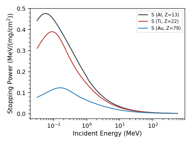
Overlaying a few elements shows the systematics — stopping falls with energy (faster particles interact less) and, per unit mass, with the atomic number of the material:
f, ax = ci.Element('Al').plot_S(return_plot=True)
ci.Element('Ti').plot_S(f=f, ax=ax)
ci.Element('Au').plot_S(f=f, ax=ax)
Ranges
Integrating the stopping power gives the range — how far the particle travels before stopping:
>>> print(el.range(15.0))       # cm
0.0871...
>>> print(10*el.range(15.0))    # mm
0.871...
A 15 MeV proton stops in under a millimeter of titanium. Numbers like these are the first sanity check of any stack design: a foil much thinner than the range perturbs the beam gently; one comparable to the range nearly stops it. Compounds work identically, with presets for common materials:
>>> cm = ci.Compound('Kapton')     # in ci.COMPOUND_LIST
>>> print(cm.density)
1.42
>>> print(cm.range(15.0))          # cm, as for elements
0.2036...
>>> print(cm.range(15.0, density=1E-3))
289.24...
The second form (the density=1E-3 idiom again) gives the range as a
areal density (mass thickness) in mg/cm2 — the unit stacked-target work is done in,
since foils are weighed rather than measured.
A first stack
Now put foils in a beam. A common pattern is repeating groups of monitor and target foils separated by degraders (a monitor foil carries a reaction whose cross section is already well known, so its measured activity determines the beam current at that position; a target foil carries the reaction under study) — here two Al–Ti–Cu groups in a 30 MeV proton beam:
stack = [{'cm':'Al', 't':0.5,   'name':'Al01'},
         {'cm':'Ti', 't':0.025, 'name':'Ti01'},
         {'cm':'Cu', 't':0.025, 'name':'Cu01'},
         {'cm':'Al', 't':0.5,   'name':'Al02'},
         {'cm':'Ti', 't':0.025, 'name':'Ti02'},
         {'cm':'Cu', 't':0.025, 'name':'Cu02'}]

st = ci.Stack(stack, E0=30.0, particle='p')
Thicknesses are in mm; Curie converts them to areal densities using each material’s preset density. The result is an energy assignment for every foil:
>>> print(st.stack)
   name compound  areal_density       mu_E     sig_E
0  Al01       Al       134.9000  29.015085  0.730443
1  Ti01       Ti        11.2975  27.935964  0.321319
2  Cu01       Cu        22.3725  27.717674  0.337406
3  Al02       Al       134.9000  26.517634  0.772389
4  Ti02       Ti        11.2975  25.357176  0.346504
5  Cu02       Cu        22.3725  25.121974  0.364116

st.plot()
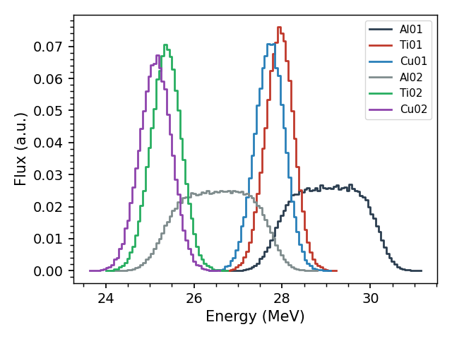
Each successive foil sees a lower mean energy. The widths follow the
foils: sig_E is dominated by how much energy the beam loses within
each foil, so the thick Al degraders show wide, path-averaged
distributions (0.73, 0.77 MeV) while the thin Ti and Cu foils record the
beam’s instantaneous spread (~0.33 MeV) at their depth.
Thin and thick foils: when the mean energy isn’t enough
It is tempting to characterize each foil by mu_E alone and read the
cross section off at that energy. For thin foils that works. For thick
foils it can fail badly, because the beam spans a wide slice of the
excitation function (the cross section as a function of energy) inside
the foil. Compare a 25 um and a 0.75 mm
titanium foil, both hit by 15 MeV protons (the range is 0.87 mm — the
thick foil absorbs most of the beam’s energy):
rx = ci.Reaction('natTI(p,x)48V')

st_thin  = ci.Stack([{'cm':'Ti', 't':0.025, 'name':'thin'}],  E0=15.0)
st_thick = ci.Stack([{'cm':'Ti', 't':0.75,  'name':'thick'}], E0=15.0)
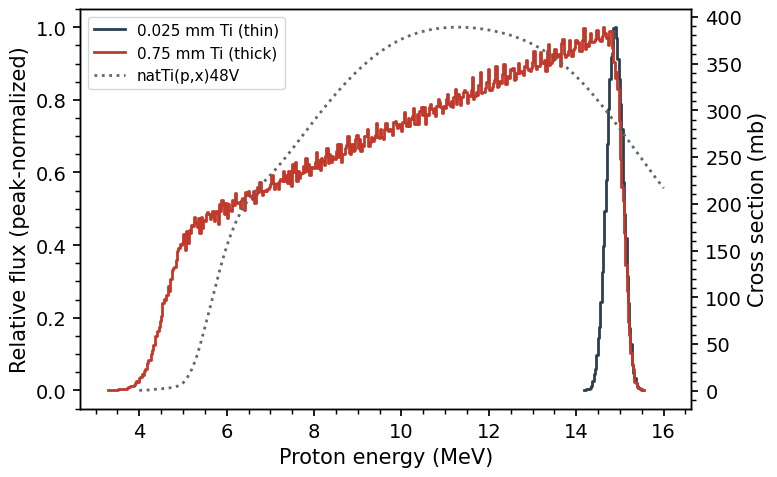
The thin foil’s flux is a narrow spike near 15 MeV; the thick foil’s stretches from 15 MeV all the way down to ~4 MeV, across the entire peak of the excitation function (dotted). Comparing the flux-averaged cross section against the shortcut of evaluating at the mean energy:
thin:  mu_E = 14.88 MeV, sig_E = 0.18 MeV
       <sigma> = 287.4 mb    sigma(mu_E) = 287.5 mb    (<0.1%)
thick: mu_E = 10.51 MeV, sig_E = 2.96 MeV
       <sigma> = 309.4 mb    sigma(mu_E) = 384.7 mb    (+24%)
computed, for each stack, as:
eng, phi = st_thin.get_flux('thin')
print(rx.average(eng, phi))                          # <sigma>
print(rx.interpolate(st_thin.stack['mu_E'][0]))      # sigma(mu_E)

eng, phi = st_thick.get_flux('thick')
print(rx.average(eng, phi))
print(rx.interpolate(st_thick.stack['mu_E'][0]))
(The figure overlays the two get_flux distributions with the
excitation function rx.interpolate on a second axis.)
For the thin foil the two agree to well under a percent; for the thick
foil the mean-energy shortcut overestimates the effective cross section
by about 24%, because the mean energy happens to sit near the peak while
much of the flux does not. (The exact Stack numbers vary slightly
run to run, since the beam energy is sampled stochastically, but this
thin-versus-thick contrast is robust.) The rule of thumb: whenever
sig_E is not small
compared to the features of the excitation function, use
rx.average(*st.get_flux(...)) — that is precisely what the flux
distributions are for.